Back To Back Leaf And Stem Plot
Kalali
Mar 24, 2025 · 6 min read
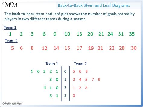
Table of Contents
Back-to-Back Leaf and Stem Plots: A Comprehensive Guide
Back-to-back stem-and-leaf plots are a powerful data visualization tool used to compare two datasets simultaneously. Unlike histograms or box plots which provide a summary view, stem-and-leaf plots offer a detailed look at the individual data points while still maintaining a clear comparison. This makes them incredibly useful for identifying patterns, trends, and outliers in paired datasets. This comprehensive guide will delve into the creation, interpretation, and applications of back-to-back stem-and-leaf plots, equipping you with the knowledge to effectively utilize this valuable statistical technique.
Understanding Stem-and-Leaf Plots: The Foundation
Before exploring back-to-back plots, it's crucial to understand the basics of a single stem-and-leaf plot. Essentially, it's a way to represent numerical data in a visually intuitive manner. Each data point is divided into two parts: a stem and a leaf.
- Stem: Represents the leading digit(s) of the data point.
- Leaf: Represents the trailing digit(s) of the data point.
For example, consider the data point 25. The stem would be 2, and the leaf would be 5.
Let's create a simple stem-and-leaf plot with the following data: 12, 15, 18, 21, 23, 29, 32, 35, 38.
| Stem | Leaf |
|---|---|
| 1 | 2 5 8 |
| 2 | 1 3 9 |
| 3 | 2 5 8 |
This plot clearly shows the distribution of the data. We can easily see the range, the clustering of data points, and any potential outliers.
Constructing Back-to-Back Stem-and-Leaf Plots: A Step-by-Step Guide
A back-to-back stem-and-leaf plot extends this concept to compare two datasets side-by-side. The stem is placed in the center, and the leaves for the first dataset are placed to the left, while the leaves for the second dataset are placed to the right.
Let's illustrate with two datasets:
Dataset A: 12, 15, 18, 21, 23, 29, 32, 35, 38 Dataset B: 19, 22, 25, 28, 31, 34, 37, 40, 42
Here's how to construct the back-to-back stem-and-leaf plot:
-
Identify the Stems: Determine the appropriate stems based on the range of values in both datasets. In this case, the stems will be 1, 2, 3, and 4.
-
Arrange the Leaves: Place the stems in a vertical column. For each data point in Dataset A, write the leaf to the left of its corresponding stem. Similarly, write the leaves for Dataset B to the right of the stem.
-
Order the Leaves: Arrange the leaves in ascending order from the stem for both datasets.
The resulting back-to-back stem-and-leaf plot would look like this:
     Dataset A     |     Dataset B
     -----------------+-----------------
        8 5 2       |       9
        9 3 1       |       8 5 2
        8 5 2       |       7 4 1 0
        | 4           |       2
     Stem | Stem
     -----------------+-----------------
             1       |       1
             2       |       2
             3       |       3
             4       |       4
Interpreting Back-to-Back Stem-and-Leaf Plots: Key Insights
Once the plot is constructed, analyzing it reveals valuable insights:
-
Comparison of Centers: By observing the distribution of leaves on either side of the stem, you can compare the central tendencies (mean, median, mode) of the two datasets. In our example, Dataset B appears to have higher values overall.
-
Comparison of Spreads: The spread (range, interquartile range, standard deviation) of each dataset can be visually assessed. The plot helps determine if one dataset is more dispersed than the other. Dataset B shows a slightly wider spread than Dataset A.
-
Identification of Outliers: Extreme values (outliers) are easily identifiable as they are significantly separated from the rest of the data points on either side. In our example, there aren't any prominent outliers.
-
Comparison of Shapes: The overall shape of the data distribution in each dataset can be compared. This helps determine if the data is symmetrical, skewed, or otherwise distributed. Both datasets in this example seem to have a somewhat right-skewed distribution.
-
Data Density: The number of leaves associated with each stem indicates data density. A higher density signifies a greater concentration of data points within that specific range.
Applications of Back-to-Back Stem-and-Leaf Plots: Real-world Scenarios
Back-to-back stem-and-leaf plots find applications in diverse fields:
-
Comparing Test Scores: Compare the performance of two different classes or groups of students on the same exam.
-
Analyzing Sales Data: Compare sales figures for two different products or regions over a specific period.
-
Evaluating Treatment Outcomes: Compare the effectiveness of two different treatments or interventions on a particular outcome variable.
-
Environmental Studies: Compare pollution levels in two different locations or over two different time periods.
-
Sports Statistics: Compare the performance metrics of two competing teams or athletes.
Advantages and Limitations of Back-to-Back Stem-and-Leaf Plots
Advantages:
- Simultaneous Comparison: Allows for a direct visual comparison of two datasets.
- Detailed Data Representation: Shows individual data points, unlike summary statistics plots.
- Easy to Construct and Understand: Relatively simple to create and interpret compared to other statistical visualizations.
- Preserves Original Data: Does not lose the raw data in the visualization.
Limitations:
- Not Suitable for Large Datasets: Becomes cumbersome and less readable with a large number of data points.
- Limited to Numerical Data: Cannot be used to visualize categorical data.
- May not be as visually appealing as other plots: Can appear less sophisticated than other visualizations like box plots.
- Requires careful consideration of stem choices: The choice of stem impacts the visual interpretation.
Choosing the Right Stem: A Critical Consideration
The choice of stem significantly influences the interpretability of the plot. If stems are too broad, the plot may not effectively highlight differences between the datasets. If stems are too narrow, the plot might become excessively spread out. Consider these strategies for effective stem selection:
- Examine the Range: Understand the minimum and maximum values in both datasets to determine the appropriate range of stems.
- Aim for a Balanced Spread: The number of leaves associated with each stem should be relatively balanced to prevent overcrowding or sparseness.
- Experiment with Different Stem Choices: If the initial stem choice results in an uninformative plot, experiment with alternative options.
Extending the Concept: Variations and Modifications
While the basic structure is straightforward, you can modify back-to-back stem-and-leaf plots to enhance clarity and detail:
- Using Different Units: If the datasets use different units, make this clear by labeling each side of the plot accordingly.
- Adding Key Information: Include a title, labels for datasets, and a key explaining the stem and leaf values.
- Highlighting Specific Values: Use different symbols or colors to highlight important data points like outliers or medians.
Conclusion: Mastering Back-to-Back Stem-and-Leaf Plots for Data Analysis
Back-to-back stem-and-leaf plots provide a unique blend of detail and comparative visualization. Their simplicity in construction belies their power in revealing insightful comparisons between two datasets. By mastering the principles outlined in this guide, you can effectively utilize this tool to enhance data analysis, communication, and decision-making. Remember to carefully consider stem selection and data representation to maximize the effectiveness of the plot and ensure clear communication of your findings. With practice, you'll find this technique invaluable in diverse analytical contexts.
Latest Posts
Latest Posts
-
How Many Liters Is 1500 Milliliters
Mar 28, 2025
-
What Percentage Is 17 Out Of 20
Mar 28, 2025
-
100 Degrees Is What In Celsius
Mar 28, 2025
-
What Is The Percentage Of 5 Out Of 6
Mar 28, 2025
-
How Many Inches Is 97 Cm
Mar 28, 2025
Related Post
Thank you for visiting our website which covers about Back To Back Leaf And Stem Plot . We hope the information provided has been useful to you. Feel free to contact us if you have any questions or need further assistance. See you next time and don't miss to bookmark.
