Finding Velocity From Position Time Graph
Kalali
Apr 07, 2025 · 6 min read
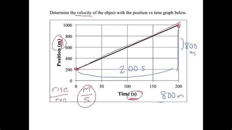
Table of Contents
Finding Velocity from a Position-Time Graph: A Comprehensive Guide
Understanding velocity and its relationship to position and time is fundamental in physics and numerous real-world applications. Whether you're analyzing the motion of a projectile, tracking the movement of a vehicle, or studying the behavior of particles, the ability to extract velocity information from a position-time graph is crucial. This comprehensive guide will walk you through the process, covering various scenarios and providing practical examples to solidify your understanding.
Understanding the Basics: Position, Time, and Velocity
Before diving into the intricacies of graph analysis, let's establish the foundational concepts:
-
Position (x or y): This represents the location of an object at a specific point in time. It's often measured relative to a reference point (e.g., origin). Units can be meters (m), kilometers (km), miles (mi), etc.
-
Time (t): This is the independent variable, representing the moment at which the position is measured. Units are typically seconds (s), minutes (min), hours (hr), etc.
-
Velocity (v): This is the rate of change of position with respect to time. It indicates both the speed and direction of motion. A positive velocity signifies movement in the positive direction, while a negative velocity indicates movement in the negative direction. Units are usually meters per second (m/s), kilometers per hour (km/h), etc.
The key relationship is that velocity is the derivative of position with respect to time. This means that the velocity at any given point can be determined by calculating the instantaneous rate of change of position.
Extracting Velocity from a Position-Time Graph: Different Approaches
Position-time graphs provide a visual representation of an object's motion. The x-axis typically represents time, and the y-axis represents position. The shape of the graph reveals valuable information about the object's velocity. Several methods exist for determining velocity from such a graph:
1. Calculating Average Velocity: The Simple Approach
The simplest way to determine velocity from a position-time graph is to calculate the average velocity over a specific time interval. This approach is suitable when you need a general overview of the object's motion, rather than precise instantaneous velocities.
Formula:
Average velocity (v<sub>avg</sub>) = (Δx) / (Δt) = (x<sub>final</sub> - x<sub>initial</sub>) / (t<sub>final</sub> - t<sub>initial</sub>)
Where:
- Δx is the change in position
- Δt is the change in time
Graphical Interpretation:
On a position-time graph, the average velocity over a given interval corresponds to the slope of the secant line connecting the two points representing the start and end of that interval. A steeper slope indicates a higher average velocity.
Example:
If an object moves from x = 5 meters at t = 1 second to x = 15 meters at t = 3 seconds, the average velocity is:
v<sub>avg</sub> = (15 m - 5 m) / (3 s - 1 s) = 10 m/2 s = 5 m/s
2. Determining Instantaneous Velocity: The Calculus Approach
For a more precise understanding of an object's motion, you need to find the instantaneous velocity. This represents the velocity at a specific point in time. This requires finding the slope of the tangent line to the curve at that point.
Graphical Interpretation:
Unlike average velocity, which uses a secant line, instantaneous velocity utilizes the tangent line. The slope of the tangent line at a specific point on the curve provides the instantaneous velocity at that exact moment.
Calculus Application:
Mathematically, instantaneous velocity is found by taking the derivative of the position function with respect to time. If the position function is denoted as x(t), then the instantaneous velocity v(t) is given by:
v(t) = dx(t)/dt
Example:
If the position function is x(t) = 2t² + 3t, then the instantaneous velocity function is:
v(t) = dx(t)/dt = 4t + 3
To find the instantaneous velocity at t = 2 seconds, substitute t = 2 into the velocity function:
v(2) = 4(2) + 3 = 11 m/s
3. Interpreting the Shape of the Curve: Qualitative Analysis
The shape of the position-time graph provides valuable qualitative information about velocity:
-
Horizontal Line: A horizontal line indicates zero velocity (object is at rest).
-
Straight Line with Positive Slope: A straight line with a positive slope indicates constant positive velocity (object moving in the positive direction at a constant speed).
-
Straight Line with Negative Slope: A straight line with a negative slope indicates constant negative velocity (object moving in the negative direction at a constant speed).
-
Curve: A curved line indicates changing velocity (object is accelerating or decelerating). The curvature indicates the rate of change of velocity (acceleration). A concave-up curve indicates positive acceleration (increasing velocity), while a concave-down curve indicates negative acceleration (decreasing velocity).
Handling Different Types of Position-Time Graphs
The techniques described above can be applied to various types of position-time graphs, including those representing:
-
Uniform Motion: These graphs display straight lines, indicating constant velocity.
-
Non-Uniform Motion: These graphs depict curves, indicating changing velocity (acceleration or deceleration).
-
Motion with Changes in Direction: These graphs may show sections with positive and negative slopes, representing changes in the direction of motion.
Advanced Considerations and Applications
Understanding velocity from position-time graphs extends beyond simple calculations. It's crucial for analyzing complex scenarios and solving real-world problems. Here are some advanced applications:
-
Determining Acceleration: The rate of change of velocity is acceleration. To find acceleration from a position-time graph, you can calculate the slope of the velocity-time graph (which can be derived from the position-time graph). Alternatively, for a position function x(t), acceleration a(t) = d²x(t)/dt².
-
Analyzing Projectile Motion: Projectile motion involves both horizontal and vertical components of velocity. Analyzing the position-time graphs for each component separately allows for a complete understanding of the projectile's trajectory.
-
Modeling Real-World Phenomena: Position-time graphs can model various phenomena, from the movement of planets to the flow of traffic. Analyzing these graphs allows for predictions and insights into the underlying processes.
-
Solving Physics Problems: Numerous physics problems involve determining velocity from a given position-time graph or equation. The techniques discussed above provide the tools to solve such problems efficiently.
Conclusion: Mastering Velocity from Position-Time Graphs
Mastering the ability to extract velocity information from position-time graphs is essential for anyone studying physics or working in related fields. This comprehensive guide has provided a thorough overview of the techniques, from calculating average velocity to determining instantaneous velocity using calculus. By understanding the relationship between position, time, and velocity, and by applying the graphical and mathematical methods outlined here, you will be well-equipped to analyze motion and solve a wide array of problems related to velocity. Remember to practice regularly to solidify your understanding and develop your analytical skills. The more you work with these graphs, the more intuitive the process will become.
Latest Posts
Latest Posts
-
How Many Days Is In 11 Weeks
Jul 14, 2025
-
How Many Grams Are In One Tola Gold
Jul 14, 2025
-
How Many Oz In A Pound Of Freon
Jul 14, 2025
-
How Many Years Are In A Millennia
Jul 14, 2025
-
Words With C As The Second Letter
Jul 14, 2025
Related Post
Thank you for visiting our website which covers about Finding Velocity From Position Time Graph . We hope the information provided has been useful to you. Feel free to contact us if you have any questions or need further assistance. See you next time and don't miss to bookmark.