How Do You Graph Tangent Functions
Kalali
Mar 28, 2025 · 5 min read
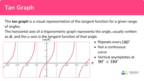
Table of Contents
How to Graph Tangent Functions: A Comprehensive Guide
The tangent function, denoted as tan(x), is a fundamental trigonometric function with unique characteristics that distinguish it from sine and cosine. Unlike sine and cosine, which have a range between -1 and 1, the tangent function has a range of all real numbers. This means the graph extends infinitely upwards and downwards. Understanding how to graph tangent functions requires grasping its key features: period, asymptotes, and its behavior within a single period. This comprehensive guide will walk you through the process step-by-step, equipping you with the skills to accurately and efficiently graph tangent functions.
Understanding the Tangent Function's Properties
Before diving into graphing, let's review the essential properties of the tangent function that influence its graphical representation:
1. Periodicity:
The tangent function is periodic, meaning its graph repeats itself at regular intervals. The period of tan(x) is π (pi) radians or 180°. This means the graph completes one full cycle every π units. This periodicity is crucial for efficiently graphing the function.
2. Asymptotes:
Unlike sine and cosine, the tangent function possesses vertical asymptotes. These are vertical lines that the graph approaches but never touches. Asymptotes occur wherever the denominator of the tangent function (cosine) equals zero. For tan(x), asymptotes occur at x = (π/2) + nπ, where 'n' is any integer. Recognizing and plotting these asymptotes is vital for an accurate graph.
3. Domain and Range:
The domain of tan(x) is all real numbers except for the values where the asymptotes occur (x ≠ (π/2) + nπ). The range, however, is all real numbers (-∞, ∞). This unbounded range indicates the graph extends infinitely in both the positive and negative y-directions.
4. Key Points:
Within a single period, there are key points that help to shape the graph. These include:
- x = 0: tan(0) = 0
- x = π/4: tan(π/4) = 1
- x = -π/4: tan(-π/4) = -1
These points, along with the asymptotes, provide a framework for sketching the curve.
Step-by-Step Guide to Graphing Tangent Functions
Now, let's proceed with a step-by-step approach to graphing tangent functions. We'll illustrate this with the example of y = tan(x).
Step 1: Identify the Period and Asymptotes
The period of y = tan(x) is π. The asymptotes occur at x = (π/2) + nπ, where n is an integer. For our initial graph, let's focus on the interval from -π/2 to π/2, encompassing one full period. Mark the asymptotes at x = -π/2 and x = π/2 on your coordinate plane. These are vertical lines that the graph will approach but never cross.
Step 2: Plot Key Points
Now, let's plot the key points within the chosen interval (-π/2, π/2):
- (0, 0): This is the point where the graph intersects the origin.
- (π/4, 1): At x = π/4, the function value is 1.
- (-π/4, -1): At x = -π/4, the function value is -1.
Plot these points on your graph.
Step 3: Sketch the Curve
Using the asymptotes and key points as guides, sketch the curve of the tangent function. The graph will increase steadily from left to right, approaching the asymptotes without ever touching them. The curve will be smooth and continuous within the interval (-π/2, π/2).
Step 4: Extend the Graph (Optional)
Since the tangent function is periodic, you can extend the graph beyond the initial period by repeating the pattern. Simply replicate the curve from (-π/2, π/2) to the left and right, ensuring that the asymptotes and key points are maintained in each successive period. This will result in a series of repeating curves.
Graphing Transformations of Tangent Functions
The basic tangent function, y = tan(x), can be transformed using various parameters. Understanding these transformations is crucial for graphing more complex tangent functions.
1. Vertical Stretching/Compression:
The equation y = A tan(x) represents a vertical stretch or compression. If |A| > 1, the graph is stretched vertically; if 0 < |A| < 1, the graph is compressed vertically. The value of A also affects the steepness of the curve.
2. Horizontal Stretching/Compression and Phase Shifts:
The equation y = tan(Bx) represents horizontal stretching/compression and phase shifts. If |B| > 1, the graph is compressed horizontally, effectively increasing the frequency of the cycles. If 0 < |B| < 1, the graph is stretched horizontally, decreasing the frequency. The period of y = tan(Bx) is π/|B|.
A phase shift (horizontal shift) is introduced by the equation y = tan(Bx - C), where C/B represents the horizontal shift.
3. Vertical Shifts:
A vertical shift is introduced by adding a constant, D, to the equation: y = tan(x) + D. This shifts the entire graph D units upwards if D > 0, and D units downwards if D < 0.
4. Combining Transformations:
Many tangent functions involve multiple transformations. To graph such functions, analyze each transformation individually and apply them in the correct order (typically, horizontal stretch/compression and phase shift first, followed by vertical stretch/compression, and finally vertical shift).
Example: Graph y = 2 tan(2x - π/2) + 1
- Period: The period is π/|B| = π/2.
- Asymptotes: The asymptotes occur when 2x - π/2 = (π/2) + nπ, which simplifies to x = π/2 + nπ/2.
- Horizontal Shift: The phase shift is C/B = (π/2)/2 = π/4 (shift to the right).
- Vertical Stretch: The amplitude is 2 (vertical stretch by a factor of 2).
- Vertical Shift: The graph is shifted 1 unit upward.
Graphing this would involve applying these transformations to the basic tan(x) graph.
Practical Applications and Further Exploration
Understanding how to graph tangent functions extends beyond theoretical exercises. It finds applications in various fields:
- Physics: Modeling oscillatory motion, such as the motion of a pendulum, often involves tangent functions.
- Engineering: Analyzing circuits and signals often utilizes trigonometric functions, including the tangent.
- Computer Graphics: Tangent functions are used in creating certain types of curves and surfaces.
Further exploration of tangent functions could include:
- Investigating the derivative and integral of the tangent function.
- Exploring the relationship between the tangent function and other trigonometric functions.
- Studying the tangent function's complex behavior in the context of complex numbers.
By mastering the techniques outlined in this guide, you'll be well-equipped to confidently tackle various problems involving tangent functions and their applications. Remember to practice regularly, and don't hesitate to consult additional resources if needed. The key to proficiency lies in understanding the fundamental properties and applying the transformation rules effectively. Through practice, graphing tangent functions will become an intuitive process.
Latest Posts
Latest Posts
-
How Much Is 25 20 Dollar Bills
Jul 05, 2025
-
How Many Apples In 3 Lb Bag
Jul 05, 2025
-
What Is Half A Quarter Of 400
Jul 05, 2025
-
How Do You Make A Vegetable Necklace
Jul 05, 2025
-
How Many 750ml Are In 1 75 Liters
Jul 05, 2025
Related Post
Thank you for visiting our website which covers about How Do You Graph Tangent Functions . We hope the information provided has been useful to you. Feel free to contact us if you have any questions or need further assistance. See you next time and don't miss to bookmark.