How To Find Velocity On A Position Time Graph
Kalali
Mar 12, 2025 · 6 min read
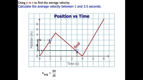
Table of Contents
How to Find Velocity on a Position-Time Graph: A Comprehensive Guide
Understanding how to extract velocity from a position-time graph is fundamental to mastering kinematics in physics. This comprehensive guide will walk you through the process, covering various scenarios and providing practical examples to solidify your understanding. We'll explore different methods, including calculating average velocity, instantaneous velocity, and handling scenarios with non-linear graphs. By the end, you'll be confident in interpreting position-time graphs and extracting meaningful information about an object's motion.
Understanding Position-Time Graphs
A position-time graph plots an object's position (often denoted as 'x' or 'y') on the vertical axis against time ('t') on the horizontal axis. The slope of the line at any point on the graph represents the object's velocity at that specific instant. This means that a steeper slope indicates a higher velocity, and a flatter slope indicates a lower velocity.
Key Features of Position-Time Graphs:
- Positive slope: Indicates positive velocity (movement in the positive direction).
- Negative slope: Indicates negative velocity (movement in the negative direction).
- Zero slope (horizontal line): Indicates zero velocity (the object is stationary).
- Curved line: Indicates changing velocity (acceleration is present).
- Straight line: Indicates constant velocity (no acceleration).
Calculating Average Velocity
The average velocity over a given time interval is calculated by finding the slope of the secant line connecting the two points on the graph representing the beginning and end of that interval.
Formula:
Average Velocity = (Change in Position) / (Change in Time) = (Δx) / (Δt)
Example:
Let's say a car's position is plotted on a graph. At time t=2 seconds, the car's position is x=10 meters. At time t=8 seconds, the car's position is x=60 meters.
Average velocity = (60 m - 10 m) / (8 s - 2 s) = 50 m / 6 s = 8.33 m/s
This means that the car's average velocity over the 6-second interval was 8.33 meters per second.
Determining Instantaneous Velocity
Instantaneous velocity represents the velocity of an object at a specific moment in time. For a position-time graph with a straight line (constant velocity), the instantaneous velocity is the same as the average velocity. However, for a curved line (changing velocity), we need to find the slope of the tangent line at the point of interest.
Finding Instantaneous Velocity Graphically:
-
Identify the point: Locate the point on the graph representing the time at which you want to find the instantaneous velocity.
-
Draw a tangent line: Draw a line that just touches the curve at that point without crossing it. This line represents the instantaneous rate of change at that precise moment. It's crucial to draw the tangent line accurately; a slight inaccuracy can significantly affect your velocity calculation.
-
Calculate the slope: Determine the slope of the tangent line using two points on the line. Use the same formula as for average velocity: (Δx) / (Δt). The slope of this tangent line is the instantaneous velocity at that specific point in time.
Finding Instantaneous Velocity with Calculus (for Advanced Users):
If you have the mathematical equation describing the position as a function of time (e.g., x(t) = 2t² + 5t), you can use calculus to find the instantaneous velocity. The instantaneous velocity is the derivative of the position function with respect to time: v(t) = dx/dt.
Example using Calculus:
If x(t) = 2t² + 5t, then v(t) = d(2t² + 5t)/dt = 4t + 5. This equation allows you to calculate the instantaneous velocity at any time 't'. For example, at t = 3 seconds, v(3) = 4(3) + 5 = 17 m/s.
Interpreting Complex Position-Time Graphs
Real-world motion is rarely represented by simple straight lines. Let's consider scenarios with more complex graphs:
Scenario 1: A Graph with Multiple Line Segments
A graph with multiple line segments indicates changes in velocity. Each segment represents a period of constant velocity. To determine the velocity during each segment, calculate the slope of that particular segment using the method for average velocity. The sign of the slope (+ or -) indicates the direction of motion.
Scenario 2: A Curved Position-Time Graph (Non-Uniform Motion)
A curved line on a position-time graph indicates that the object is accelerating (its velocity is changing). The curvature indicates the rate of acceleration. A steeper curve suggests a greater acceleration (or deceleration, if the curve is downward). Remember, the instantaneous velocity at any point is given by the slope of the tangent line at that point.
Scenario 3: A Graph Showing Rest Periods
A horizontal line segment on a position-time graph signifies that the object is at rest (zero velocity). The length of the horizontal segment indicates the duration of the rest period.
Scenario 4: Graphs with Discontinuities
In certain situations, the graph might show a sudden jump or discontinuity. This might represent an instantaneous change in position (e.g., a teleportation scenario in a thought experiment, or a more realistic example like an object being abruptly moved). Calculating the velocity across such a discontinuity is not meaningful as it involves an infinite rate of change. Focus instead on the velocity before and after the jump.
Practical Applications and Tips
Understanding velocity from position-time graphs has numerous practical applications, including:
- Analyzing the motion of vehicles: Determining speeds and accelerations of cars, trains, or airplanes.
- Studying projectile motion: Calculating the velocity of a ball thrown into the air.
- Understanding population dynamics: Modeling population growth or decline over time.
- Analyzing economic trends: Studying changes in economic indicators over time.
Tips for Success:
- Practice regularly: The more you practice interpreting position-time graphs, the better you'll become at it.
- Pay attention to units: Always remember to include the appropriate units (e.g., m/s, km/h) in your calculations.
- Use appropriate tools: A ruler or straight edge is helpful for drawing tangent lines accurately. Graphing software can also be beneficial for analyzing complex graphs.
- Understand the context: Consider the physical situation represented by the graph. This will help you interpret the results meaningfully.
- Break down complex graphs: If a graph is complex, break it down into smaller, simpler segments to analyze it more easily.
Conclusion
Mastering the interpretation of position-time graphs is a crucial skill in physics and related fields. By understanding how to calculate average and instantaneous velocities, interpret different graph shapes, and handle complex scenarios, you can gain valuable insights into the motion of objects and systems. Remember that practice and careful attention to detail are key to achieving proficiency in this essential area. Continue practicing with various graph types and examples to solidify your understanding and improve your analytical abilities.
Latest Posts
Latest Posts
-
If Your 35 What Year Was You Born
Jul 12, 2025
-
How Many Cups Is 1 Pound Of Cheese
Jul 12, 2025
-
30 X 30 Is How Many Square Feet
Jul 12, 2025
-
How Much Does A Half Oz Weigh
Jul 12, 2025
-
Calories In An Omelette With 3 Eggs
Jul 12, 2025
Related Post
Thank you for visiting our website which covers about How To Find Velocity On A Position Time Graph . We hope the information provided has been useful to you. Feel free to contact us if you have any questions or need further assistance. See you next time and don't miss to bookmark.