A Velocity Time Graph Shows How Velocity Changes Over
Kalali
Mar 25, 2025 · 6 min read
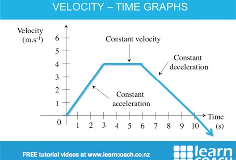
Table of Contents
Velocity-Time Graphs: Decoding the Motion of Objects
A velocity-time graph is a powerful tool used in physics and engineering to visually represent how the velocity of an object changes over time. Understanding how to interpret these graphs is crucial for analyzing motion and solving kinematic problems. This comprehensive guide will delve into the intricacies of velocity-time graphs, exploring their construction, interpretation, and application in various scenarios. We'll cover key concepts like calculating acceleration, displacement, and identifying different types of motion depicted in these graphs.
Understanding the Axes and Data Representation
Before diving into the complexities, let's establish the basics. A velocity-time graph plots velocity on the y-axis (vertical axis) and time on the x-axis (horizontal axis). The velocity is usually expressed in units like meters per second (m/s), kilometers per hour (km/h), or miles per hour (mph), while time is measured in seconds (s), minutes (min), or hours (h). Each point on the graph represents the object's velocity at a specific moment in time.
Key Features to Look For:
-
Slope: The slope of the line on a velocity-time graph represents the acceleration of the object. A positive slope indicates positive acceleration (increasing velocity), a negative slope indicates negative acceleration (decreasing velocity or deceleration), and a zero slope (horizontal line) indicates zero acceleration (constant velocity).
-
Area Under the Curve: The area under the curve of a velocity-time graph represents the displacement of the object. This is the net change in position from the starting point. For simple shapes like rectangles and triangles, calculating the area is straightforward. For more complex curves, integration techniques may be necessary.
-
Intercepts: The y-intercept (where the line crosses the y-axis) represents the object's initial velocity at time t=0. The x-intercept (where the line crosses the x-axis) represents the time at which the object's velocity is zero.
Interpreting Different Types of Motion
Velocity-time graphs can represent various types of motion, each characterized by a distinct graphical representation:
1. Uniform Motion (Constant Velocity)
In uniform motion, the object moves at a constant velocity. This is represented by a horizontal straight line on the velocity-time graph. The slope of the line is zero, indicating zero acceleration. The displacement is simply the velocity multiplied by the time elapsed.
2. Uniformly Accelerated Motion
Uniformly accelerated motion describes an object moving with a constant acceleration. This is represented by a straight line with a non-zero slope on the velocity-time graph. The slope of the line represents the constant acceleration. The displacement can be calculated using kinematic equations or by finding the area under the line.
- Positive Acceleration: A line sloping upwards indicates positive acceleration (increasing velocity).
- Negative Acceleration (Deceleration): A line sloping downwards indicates negative acceleration (decreasing velocity).
3. Non-Uniformly Accelerated Motion
In non-uniformly accelerated motion, the acceleration of the object is not constant. This is represented by a curved line on the velocity-time graph. The slope of the tangent to the curve at any point represents the instantaneous acceleration at that point. Calculating the displacement requires more complex methods, often involving integration.
4. Motion with Changing Acceleration
This is a more complex scenario where the acceleration itself changes over time. The graph will be a curve, and the slope of the tangent at any point gives the instantaneous acceleration. Determining the displacement will necessitate calculus to calculate the area under the curve. This might involve numerical integration techniques if an analytical solution is not readily available.
Calculating Key Parameters from Velocity-Time Graphs
Velocity-time graphs provide a convenient way to calculate various parameters related to an object's motion:
1. Calculating Acceleration
As previously stated, the slope of the line (or tangent to the curve) on a velocity-time graph represents the acceleration. The formula for calculating the slope is:
Acceleration (a) = (Change in velocity) / (Change in time) = (v₂ - v₁) / (t₂ - t₁)
Where:
- v₂ is the final velocity
- v₁ is the initial velocity
- t₂ is the final time
- t₁ is the initial time
2. Calculating Displacement
The area under the curve of a velocity-time graph represents the displacement of the object. For simple shapes like rectangles and triangles, the area can be easily calculated using standard geometric formulas. For more complex shapes, integration techniques are required.
- Rectangular Area: Area = base × height = time × velocity
- Triangular Area: Area = (1/2) × base × height = (1/2) × time × change in velocity
For irregular shapes, numerical integration methods, such as the trapezoidal rule or Simpson's rule, can provide an approximation of the area and therefore the displacement.
3. Determining the Instantaneous Velocity
The instantaneous velocity at any point in time is simply the y-coordinate (velocity value) at that specific time on the graph.
Advanced Applications and Considerations
Velocity-time graphs are not limited to simple motion analysis. They have broader applications, including:
- Analyzing projectile motion: Velocity-time graphs can effectively illustrate the vertical and horizontal components of velocity in projectile motion.
- Studying collisions: The changes in velocity during collisions can be easily visualized and analyzed using velocity-time graphs.
- Understanding braking distances: These graphs can be used to calculate stopping distances, vital in transportation safety.
- Investigating the motion of complex systems: In more advanced physics, velocity-time graphs help visualize the motion of systems with multiple interacting objects.
While analyzing velocity-time graphs, it's essential to consider the following:
- Units: Always pay close attention to the units used for velocity and time. Inconsistent units can lead to inaccurate calculations.
- Scale: The scale of the axes significantly impacts the graph's appearance and interpretation.
- Assumptions: The analysis often relies on certain assumptions, such as neglecting air resistance or considering the object as a point mass.
Conclusion
Velocity-time graphs offer a powerful and intuitive visual representation of an object's motion. By understanding how to interpret the slope, area under the curve, and various graph shapes, we can extract valuable information about acceleration, displacement, and the nature of the motion itself. Mastering the skills of interpreting and constructing these graphs is a cornerstone of understanding kinematics and is applicable across many scientific and engineering disciplines. From simple scenarios to more complex systems, velocity-time graphs provide a clear and effective means of visualizing and quantifying motion. The ability to accurately interpret these graphs is crucial for problem-solving and developing a deep understanding of classical mechanics. Therefore, a thorough comprehension of this tool remains a valuable asset in any scientific or engineering pursuit.
Latest Posts
Latest Posts
-
How Many Centimeters Is 15 In
Mar 26, 2025
-
How To Use Pascals Triangle To Expand Polynomials
Mar 26, 2025
-
How Do The Inner Planets Differ From The Outer Planets
Mar 26, 2025
-
Words Where W Is A Vowel
Mar 26, 2025
-
How Does The Muscular System Maintain Homeostasis
Mar 26, 2025
Related Post
Thank you for visiting our website which covers about A Velocity Time Graph Shows How Velocity Changes Over . We hope the information provided has been useful to you. Feel free to contact us if you have any questions or need further assistance. See you next time and don't miss to bookmark.
